
Join us on our journey towards renewable energy excellence, where knowledge meets innovation.

The introduction of Redispatch 2.0 on October 1, 2021, fundamentally restructured how grid operators and plant operators in Germany manage congestion and compensate for curtailed energy. For renewable systems (solar and wind) with a nominal capacity of 100 kW or more, the regulatory framework established by the Federal Network Agency (BK6-20-059, Annex 1) defines three distinct methodologies for determining lost work, i.e. the energy not fed into the grid during a redispatch measure: peak (Spitz), simplified peak (Spitz-light) and flat-rate (Pauschal).
Each method employs a different approach to estimating the theoretical feed-in that would have occurred absent the curtailment. The choice between them, which operators must make annually by November 30, carries direct economic consequences: the calculated lost work forms the basis for compensation.
This article examines these three settlement methods from a technical perspective. For each method, we walk through the calculation step by step, showing exactly which data inputs are required and how they are combined to determine lost work.
We then present illustrative examples comparing the flat-rate and simplified peak methods for a hypothetical 100 MWp solar plant, demonstrating how the choice of method can lead to significantly different outcomes depending on the season and weather conditions.


Before examining each settlement method individually, it is useful to understand the fundamental calculation that underpins all three approaches. For any given 15-minute interval during a redispatch measure, lost work is determined as:

W_A,i : Lost work in quarter-hour i (kWh).
P_est,i : Estimated theoretical feed-in in quarter- hour i (kW).
P_lim,i :Power limit imposed by the grid operator in quarter-hour i (kW).
The logic is straightforward: if the estimated theoretical feed-in exceeds the allowed limit, the difference represents energy that was curtailed and must be compensated. The factor ¼ h converts the power difference (kW) into energy (kWh) for the 15-minute interval.
The common framework above applies to all three settlement methods. Where they differ is in how P_est,i, the estimated feed-in during the redispatch measure, is determined.

In all methods, the calculated theoretical feed-in is capped at the plant's nominal capacity. If the formula yields a value above this limit, it is reduced accordingly.
The peak settlement (Spitzabrechnung) for solar calculates theoretical feed-in using on-site irradiance measurement. It relies on a specific performance ratio derived from a recent reference day to estimate what the plant would have produced during a redispatch measure.

P_VZ,ist: Average actual feed-in during the reference period (kW).
G_VZ: Average irradiance during the reference period (kW/m2).
G_i: Average irradiance during quarter-hour i of the redispatch measure (kW/m2).
The term P_VZ,ist / G_VZ represents the plant's performance ratio: its efficiency in converting irradiance to power, as observed on the most recent preceding day on which no redispatch measures occurred for the plant.
This method requires the plant to be equipped with a suitable irradiance sensor. The measured irradiance must accurately reflect the conditions at the module plane, and the sensor setup must remain consistent between the reference day and the redispatch day.
The peak settlement for wind calculates theoretical feed-in using on-site wind speed measurement at the nacelle or rotor hub. Unlike solar, which uses a performance ratio from a reference day, wind uses a correction factor derived from the last four undisturbed quarter-hours immediately before the redispatch measure.

P_vor,ist: Average actual feed-in during the last four full quarter-hours before the redispatch measure (kW).
P_vor,theo: Average theoretical power during those same four quarter-hours before the redispatch measure (kW).
P_theo,i : Average theoretical power during the quarter-hour of the redispatch measure (kW).
Theoretical power is calculated from measured wind speed and the certified power curve of the wind turbine. This requires the turbine to be equipped with a wind speed sensor (nacelle or rotor hub) and have a certified power curve available for converting measured wind speeds to theoretical power.
The simplified peak settlement (vereinfachte Spitzabrechnung) for solar follows the same calculation logic as the peak settlement but replaces on-site irradiance measurements with data from a weather data provider.
Weather data providers typically deliver horizontal irradiance values. These must be converted to plane-of-array (PoA) irradiance using the plant's location and orientation.
Simplified peak offers a middle ground: it avoids the need for on-site sensors but relies on weather data that must be converted to the module plane, introducing potential sources of error compared to direct measurement.
The simplified peak settlement for wind follows the same calculation logic as the peak settlement but replaces on-site wind speed measurements with data from a weather data provider or a suitable reference plant.
Weather data providers deliver wind speed values that must be representative of the turbine's hub height and location. For reference plants, the selected turbine must be in close spatial proximity with similar structural characteristics and terrain.
The flat-rate settlement (Pauschal-Abrechnung) for solar is used whenever quarter-hour specific measurements are unavailable to determine the theoretical performance. Instead of using real-time weather, it uses a fixed Plant Factor (AF) to estimate the theoretical output.
AF : Plant factor determined based on the season and time of day, according to the table below.
P_inst: Installed nominal capacity of the plant (kW).
Determination of the Plant Factor (AF):
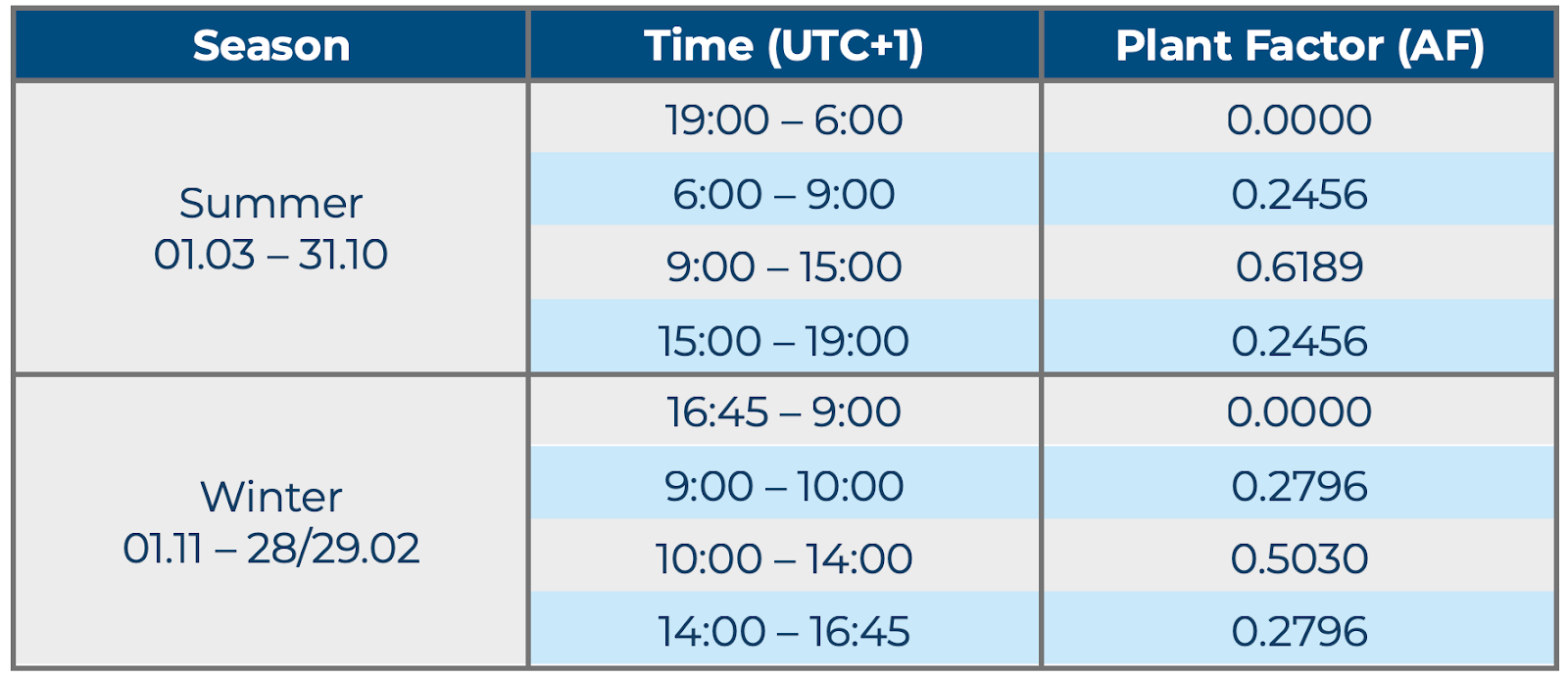
Because the plant factor is fixed by season and time of day, the flat-rate method does not respond to actual weather conditions. On a cloudy day, it may overestimate theoretical feed-in (and thus lost work), while on a particularly sunny day it may underestimate it. The method provides predictability and simplicity, but at the cost of accuracy compared to the peak-based methods.
The flat-rate settlement for wind calculates lost work based on a snapshot of the plant's output immediately before the redispatch intervention. It assumes a constant power level for the duration of the redispatch measure.

P_0: Average actual power measured during the last full quarter-hour of unrestricted operation prior to the redispatch measure (kW).
Unlike solar, which uses fixed time-of-day factors, wind flat-rate simply extrapolates the last measured value. This assumes wind conditions remain constant throughout the redispatch event, an assumption that becomes less accurate for longer durations. If no quarter-hour measurement is available for P_0, it is determined using standard or day-dependent feed-in profiles.
To show how these methods diverge in practice, we compare the flat-rate and simplified peak methods for a hypothetical 100 MWp solar plant in Germany. We selected four representative days in 2025: 1 February (winter), 1 May (spring), 1 August (summer) and 1 November (autumn).
For each day, we assume a full redispatch curtailment, meaning the power limit P_lim,i is set to zero throughout daylight hours. Under this assumption, lost work in each 15-minute interval equals the theoretical feed-in (in kW) converted to energy (in kWh) using the ¼ h factor.
For the flat-rate method, theoretical feed-in is calculated using the fixed time-of-day factors for the appropriate season, multiplied by the plant's installed capacity. For the simplified peak method, we derive a performance ratio from the previous day (assumed to be undisturbed by redispatch) and apply it to irradiance data from a weather provider, converted to the plane-of-array. All calculations are performed for each 15-minute interval.
The results for the four days are shown below.

The four plots reveal the fundamental difference between the two methods. The flat-rate method produces the same fixed profile for all days within a given season. February and November share identical stepped shapes, as do May and August. This profile is entirely deterministic, changing only with the calendar.
The simplified peak method, by contrast, responds to actual weather. May shows a near-perfect clear sky day: the simplified peak follows a smooth bell curve, the theoretical ideal that flat-rate approximates with its stepped blocks. August, while more variable, still operates at a magnitude where the two methods broadly align.
The contrast is starker in the winter plots. February captures a moderately cloudy day: simplified peak fluctuates throughout, sometimes exceeding the flat-rate estimate, sometimes falling below. November shows an overcast day with persistently low irradiance. Here, simplified peak consistently underperforms the flat-rate profile, revealing how the fixed method can significantly overestimate lost work when conditions are poor.
Together, the examples illustrate that simplified peak captures weather-driven variability while flat-rate offers a stylized, season-dependent baseline. Which method yields higher compensation depends entirely on actual conditions at the time of redispatch. Operators choose their method in November, without knowing when those events will occur. A year with many clear-sky redispatch hours will tend to favor simplified peak; a year with many overcast hours will tend to favor flat-rate. The examples above show the range of possible outcomes, but they do not imply that one method is inherently more favorable than the other.
The three settlement methods under Redispatch 2.0 offer different trade-offs between accuracy, complexity, and data requirements. Peak settlement provides the most precise estimate of lost work but requires on-site measurement equipment. Simplified peak balances accuracy with practicality by using weather data, though it introduces additional steps and potential sources of error. Flat-rate settlement is the simplest and requires no weather data, but its fixed profile cannot capture day-to-day weather variability.
For plant operators, the annual November 30 deadline is not merely administrative, it is a strategic decision with direct financial implications. The examples above show that the choice of method can materially affect compensation, but which method performs better in any given year depends on factors outside the operator's control: the timing of redispatch events and the weather on those days. Understanding how each method works is essential to making an informed choice.

 4 min
4 min

Insights, Market-trends
12th Jun, 2026
8 min
Insights, Market-trends
11th Jun, 2026
6 min

Insights
1st Jun, 2026